It’s Oscars season again so why not explore how predictable (my) movie tastes are. This has literally been a million dollar problem and obviously I am not gonna solve it here, but it’s fun and slightly educational to do some number crunching, so why not. Below, I will proceed from a simple linear regression to a generalized additive model to an ordered logistic regression analysis. And I will illustrate the results with nice plots along the way. Of course, all done in R (you can get the script here).
Data
The data for this little project comes from the IMDb website and, in particular, from my personal ratings of 442 titles recorded there. IMDb keeps the movies you have rated in a nice little table which includes information on the movie title, director, duration, year of release, genre, IMDb rating, and a few other less interesting variables. Conveniently, you can export the data directly as a csv file.
Outcome variable
The outcome variable that I want to predict is my personal movie rating. IMDb lets you score movies with one to ten stars. Half-points and other fractions are not allowed. It is a tricky variable to work with. It is obviously not a continuous one; at the same time ten ordered categories are a bit too many to treat as a regular categorical variable. Figure 1 plots the frequency distribution (black bars) and density (red area) of my ratings and the density of the IMDb scores (in blue) for the 442 observations in the data.
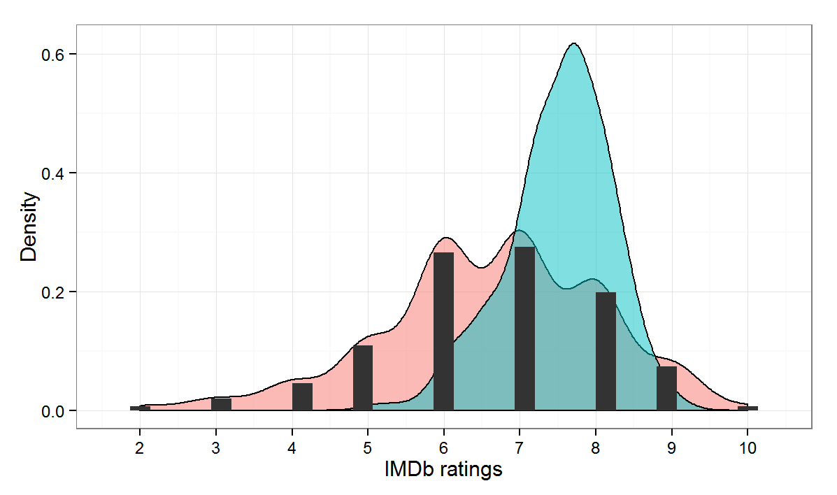
The mean of my ratings is a good 0.9 points lower than the IMDb scores, which are also less dispersed and have a higher peak (can you say ‘kurtosis’).
Data-generating process
Some reflection on how the data is generated can highlight its potential shortcomings. First, life is short and I try not to waste my time watching bad movies. Second, even if I get fooled to start watching a bad movie, usually I would not bother rating it on IMDb.There are occasional two- and three-star scores, but these are usually movies that were terrible and annoyed me for some reason or another (like, for example, getting a Cannes award or featuring Bill Murray). The data-generating process leads to a selection bias with two important implications. First, the effective range of variation of both the outcome and the main predictor variables is restricted, giving the models less information to work with. Second, because movies with a decent IMDb ratings which I disliked have a lower chance of being recorded in the dataset, the relationship we find in the sample will overestimate the real link between my ratings and the IMDb ones.
Take one: linear regression
Enough preliminaries, let’s get to business. An ordinary linear regression model is a common starting point for analysis and its results can serve as a baseline. Here are the estimates that lm provides for regressing my ratings on IMDb scores:
summary(lm(mine~imdb, data=d))

Coefficients:
            Estimate Std. Error t value Pr(>|t|)
(Intercept)  -0.6387     0.6669  -0.958    0.339
imdb          0.9686     0.0884  10.957   ***
---
Residual standard error: 1.254 on 420 degrees of freedom
Multiple R-squared: 0.2223,	Adjusted R-squared: 0.2205
The intercept indicates that on average my ratings are more than half a point lower. The positive coefficient of IMDb score is positive and very close to one which implies that one point higher (lower) IMDb rating would predict, on average, one point higher (lower) personal rating. Figure 2 plots the relationship between the two variables (for an interactive version of the scatter plot, click here):
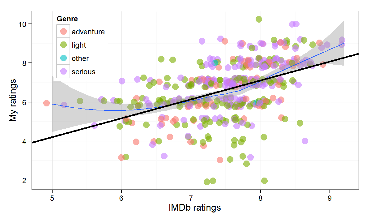
The solid black line is the regression fit, the blue one shows a non-parametric loess smoothing which suggests some non-linearity in the relationship that we will explore later.
Although the IMDb score coefficient is highly statistically significant that should not fool us that we have gained much predictive capacity. The model fit is rather poor. The root mean squared error is 1.25 which is large given the variation in the data. But the inadequate fit is most clearly visible if we plot the actual data versus the predictions. Figure 3 below does just that. The grey bars show the prediction plus/minus two predictive standard errors. If the predictions derived from the model were good, the dots (observations) would be very close to the diagonal (indicated by the dotted line). In this case, they are not. The model does a particularly bad job in predicting very low and very high ratings.

We can also see how little information IMDb scores contain about (my) personal scores by going back to the raw data. Figure 4 plots to density of my ratings for two sets of values of IMDb scores – from 6.5 to 7.5 (blue) and from 7.5- to 8.5 (red). The means for the two sets differ somewhat, but the overlap in the density is great.
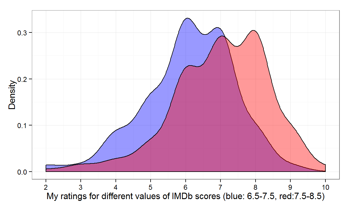
In sum, knowing the IMDb rating provides some information but on its own doesn’t get us very far in predicting what my score would be.
Take two: adding predictors
Let’s add more variables to see if things improve. Some playing around shows that among the available candidates only the year of release of the movie and dummies for a few genres and directors (selected only from those with more than four movies in the data) give any leverage.
 summary(lm(mine~imdb+d$comedy +d$romance+d$mystery+d$"Stanley Kubrick"+d$"Lars Von Trier"+d$"Darren Aronofsky"+year.c, data=d))

Coefficients:
                      Estimate Std. Error t value Pr(>|t|)
(Intercept)           1.074930   0.651223   1.651  .
imdb                  0.727829   0.087238   8.343  ***
d$comedy             -0.598040   0.133533  -4.479  ***
d$romance            -0.411929   0.141274  -2.916  **
d$mystery             0.315991   0.185906   1.700  .
d$"Stanley Kubrick"   1.066991   0.450826   2.367  *
d$"Lars Von Trier"    2.117281   0.582790   3.633  ***
d$"Darren Aronofsky"  1.357664   0.584179   2.324  *
year.c                0.016578   0.003693   4.488  ***
---
Residual standard error: 1.156 on 413 degrees of freedom
Multiple R-squared: 0.3508,	Adjusted R-squared: 0.3382
The fit improves somewhat. The root mean squared error of this model is 1.14. Moreover, looking again at the actual versus predicted ratings, the fit is better, especially for highly rated movies – no surprise given that the director dummies pick these up.

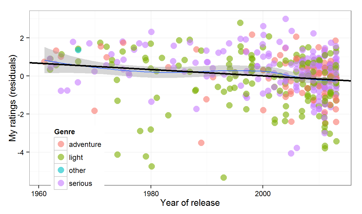
The last variable in the regression above is the year of release of the movie. It is coded as the difference from 2014, so the positive coefficient implies that older movies get higher ratings. The statistically significant effect, however, has no straightforward predictive interpretation. The reason is again selection bias. I have only watched movies released before the 1990s that have withstood the test of time. So even though in the sample older films have higher scores, it is highly unlikely that if I pick a random film made in the 1970s I would like it more than a random film made after 2010. In any case, Figure 6 below plots the year of release versus the residuals from the regression of my ratings on IMDb scores (for the subset of films after 1960). We can see that the relationship is likely nonlinear (and that I really dislike comedies from the 1980s).
So far both regressions assumed that the relationship between the predictors and the outcome is linear. Needless to say, there is no compelling reason why this should be the case. Maybe our predictions will improve if we allow the relationships to take any form. This calls for a generalized additive model.
Take three: generalized additive model (GAM)
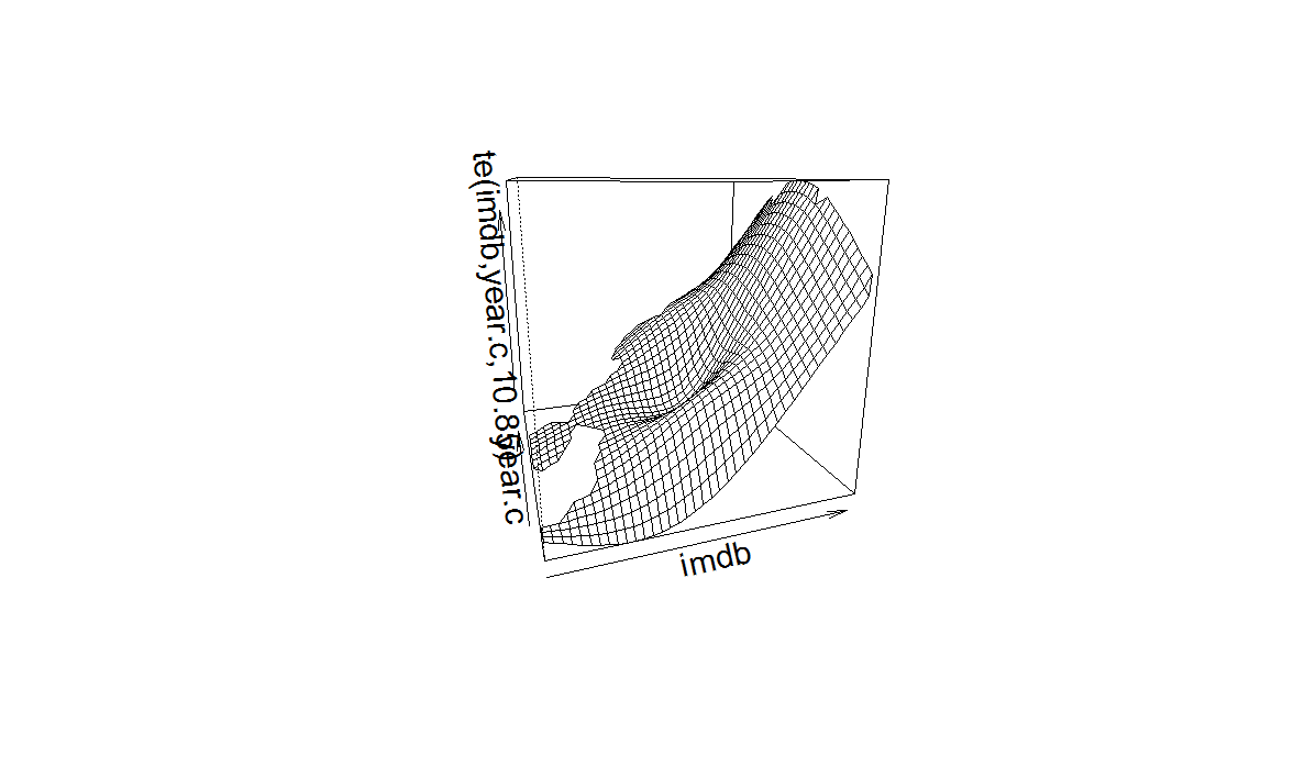
In R, we can use the mgcv library to fit a GAM. It doesn’t make sense to hypothesize non-linear effects for binary variables, so we only smooth the effects of IMDb rating and year of release. But why stop there, perhaps the non-linear effects of IMDb rating and release year are not independent, why not allow them to interact!
library(mgcv)
summary(gam(mine ~ te(imdb,year.c)+d$"comedy " +d$"romance "+d$"mystery "+d$"Stanley Kubrick"+d$"Lars Von Trier"+d$"Darren Aronofsky", data = d))

PParametric coefficients:
                     Estimate Std. Error t value Pr(|t|)
(Intercept)           6.80394    0.07541  90.225   ***
d$"comedy "          -0.60742    0.13254  -4.583   ***
d$"romance "         -0.43808    0.14133  -3.100   **
d$"mystery "          0.32299    0.18331   1.762   .
d$"Stanley Kubrick"   0.83139    0.45208   1.839   .
d$"Lars Von Trier"    2.00522    0.57873   3.465   ***
d$"Darren Aronofsky"  1.26903    0.57525   2.206   *
---
Approximate significance of smooth terms:
                  edf Ref.df     F p-value
te(imdb,year.c) 10.85  13.42 11.09
Well, the root mean squared error drops to 1.11 and the jointly smoothed (with a full tensor product smooth) variables are significant, but the added predictive value is minimal in this case. Nevertheless, the plot below shows the smoothed terms are more appropriate than the linear ones, and that there is a complex interaction between the two:
Take four: models for categorical data
So far we treated personal movie ratings as if they were a continuous variable, but they are not – taking into account that they are essentially an ordered categorical variable might help. But ten categories, while possible to model, would make the analysis rather unwieldy, so we recode the personal ratings into five categories without much loss of information: 5 and less, 6,7,8,9 and more.
We can first see a nonparametric conditional destiny plot of the newly created categorical variable as a function of IMDb scores:
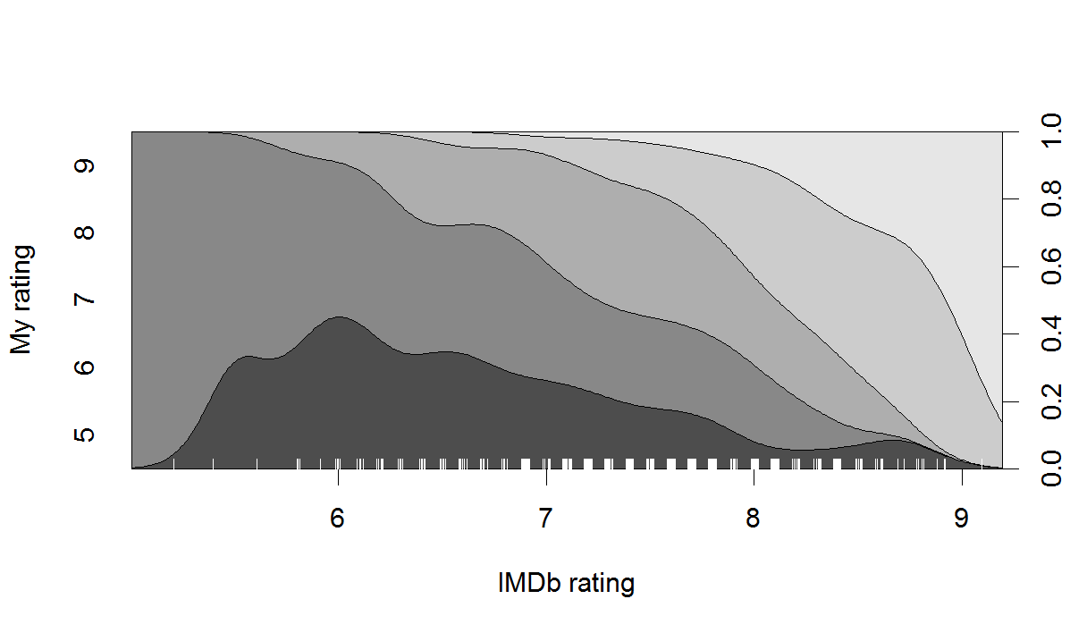
The plot shows the observed density for each category of the outcome variable along the range of the predictor. For example, for a film with an IMDb rating of ‘6’, about 35% of the personal scores are ‘5’, a further 50% are ‘6’, and the remaining 15% are ‘7’. Remember that the plot is based on the observed conditional frequencies only (with some smoothing), not on the projections of a model. But the small ups and downs seem pretty idiosyncratic. We can also fit an ordered logistic regression model, which would be appropriated for the categorical outcome variable we have, and plot its predicted probabilities given the model.
First, here is the output of the model:
library(MASS)
summary(polr(as.factor(mine.c) ~ imdb+year.c,  Hess=TRUE, data = d)
Coefficients:
        Value Std. Error t value
imdb   1.4103   0.149921   9.407
year.c 0.0283   0.006023   4.699

Intercepts:
    Value   Std. Error t value
5|6  9.0487  1.0795     8.3822
6|7 10.6143  1.1075     9.5840
7|8 12.1539  1.1435    10.6289
8|9 14.0234  1.1876    11.8079

Residual Deviance: 1148.665
AIC: 1160.665
The coefficients of the two predictors are significant. The plot below shows the predicted probability of the outcome variable – personal movie rating – being in each of the five categories as a function of IMDb rating and illustrates the substantive scale of the effect.

Compared to the non-parametric conditional density plot above, these model-based predictions are much smoother and have ‘disciplined’ the effect of the predictor to follow a systematic pattern.
It is interesting to ponder which of the two would be more useful for out-of-sample predictions. Despite the fact that the non-parametric one is more faithful to the current data, I think I would go for the parametric model projections. After all, is it really plausible that a random film with an IMDb rating of 5 would have lower chance a getting a 5 from me than a film with an IMDb rating of 6, as the non-parametric conditional density plot suggests? I don’t think so. Interestingly, in this case the parametric model has actually corrected for some of the selection bias and made for more plausible out-of-sample predictions.
Conclusion
In sum, whatever the method, it is not very fruitful to try to predict how much a person (or at least, the particular person writing this) would like a movie based on the average rating the movie gets and covariates like the genre or the director. Non-linear regressions and other modeling tricks offer only marginal predictive improvements over a simple linear regression approach, but bring plenty of insight about the data itself.
What is the way ahead? Obviously, one would want to get more relevant predictors, but, unfortunately, IMDb seems to have a policy against web-scrapping from its database, so one would either have to ask for permission or look at a different website with a more liberal policy (like Rotten Tomatoes perhaps). For me, the purpose of this exercise has been mostly in its methodological educational value, so I think I will leave it at that. Finally, don’t forget to check out the interactive scatterplot of the data used here which shows a user’s entire movie rating history at a glance.
Endnote
As you would have noted, the IMDb ratings come at a greater level of precision (like 7.3) than the one available for individual users (like 7). So a user who really thinks that a film is worth 7.5 has to pick 7 or 8, but its average IMDb score could well be 7.5. If the rating categories available to the user are indeed too coarse, this would show up in the relationship with the IMDb score: movies with an average score of 7.5 would be less predictable that movies with an average score of either 7 or 8. To test this conjecture, a rerun the linear regression models on two subsets of the data: one comprising the movies with an average IMDb rating between 5.9 and 6.1, 6.9 an 7.1, etc., and a second one comprising those with an average IMDb rating between 5.4 and 5.6, 6.4 and 6.6, etc. The fit of the regression for the first group was better than for the second (RMSE of 1.07 vs. 1.11), but, frankly, I expected a more dramatic difference. So maybe ten categories are just enough.
[…] article was first published on Rules of Reason » R, and kindly contributed to […]
Hi: Your post about the movie ratings is interesting but there are well known methods for predicting movie ratings. ( you include other people’s ratings rather than just yours ). The netflix competition spurred a lot of interest in this area. Since you didn’t use the popular method, I’m not sure if you’re aware of it ( apologies, if you are ) but it’s called “collaborative” filtering and imathematically involves the notion of matrix factorization. A while back ( couple of years ago actually ), tried to write specialized R code for the algorithm in order to handle a popular big data set ( because optimization techniques in R start bogging down when dealing with big data sets ) but I was never quite successful. Trevor hastie has recently written an R package for dealing with the problem but I forget the name of it. Anyway, there is tons of info on the net about collaborative filtering/matrix factorization in case you want to check it out. Still, thanks for your post. It was definitely interesting and creative.
Mark
thanks for your comment Mark. I am aware of the Netflix challenge (and actually link to it in the first paragraph), but there is one aspect I don’t quite understand: The winning team had to improve on the prediction (RMSE) given by a baseline model by 10% to scoop the cash (which they did in 2009). Does this mean that a common approach like a linear regression or a simple GAM gets you 99% of the way for 1% of the effort, and then the other 99% of the effort go into improving marginally on the ‘baseline’? A 10% improvement on the prediction error (RMSE) could still be important if the context involves really high stakes or billions of small-stakes decisions, but it certainly seems trivial from a more casual perspective.
In an case, getting other people’s ratings can get you into trouble – it seems that even netflix was sued for making user data available for the prediction challenge 😉
Hi Dimiter: I didn’t participate in thew netflix comp so I’m not so knowledgeable of the
details of it. I got into the NetFlix problem while taking Andrew Ng’s class where he covered it briefly. So, for fun, I was trying to use R to solve one of the problems on a medium sized Movie Lens data set which led to me getting more into the problem and it went like that.
But I clicked on your link ( sorry I missed it earlier ) and it said below:
“Using only the training data, Cinematch scores an RMSE of 0.9514 on the quiz data, roughly a 10% improvement over the trivial algorithm. Cinematch has a similar performance on the test set, 0.9525. In order to win the grand prize of $1,000,000, a participating team had to improve this by another 10%, to achieve 0.8572 on the test set.[1] Such an improvement on the quiz set corresponds to an RMSE of 0.8563”.
But a 10 percent RMSE reduction is not negligible because the Root Mean Square Error
is divided by n ( or n -1 ) I forget ) and there were 1000’s of predictions if not 10’s of thousands
or 100’s of thousands. So, to reduce the RMSE by 10% , means a lot. It sort of means that instead of the average error ( I think the ratings scale was 1 to 5 ) being 0.95 it has to be come 0.85. but that’s the average error over ALL THE PREDICTIONS.
as far as data sets go, yes, I heard that there was a problem with the Netflix data set
and they had to take it down. But when I was working on it, I used the data sets from MovieLens instead. The biggest one from MovieLens was a pretty good size but not the size of Netflix. The standard R type optimizers still had trouble with the biggest MovieLens data set. ( I remember
the one that showed the most promise was Rcgmin ) . I think KDDCUP is the data set that researchers use now instead of netflix.
I’d like to get back to the problem someday. I got somewhat demotivated because, while
I was working on it, Trevor Hastie et al came out with an R package ( forget the name ) for
Matrix Factorization kind of specifically designed for collaborative filtering that is really state of the art in terms of computational efficiency and I think handles large data sets etc. I’m not absolute sure about the “handles large data sets part” but computationally speaking, it’s definitely gonna top notch. Hastie and his group are tops in the world when it comes to these
types of problems. I hope this info clarifies or helps.
[…] Outro divertido. […]
Good work — refreshing and informative to see a case study like this. I’d like to see more of them, here or elsewhere. Any pointers?
Great post! Thank you so much for sharing..
For those who want to learn R Programming, here is a great new course on youtube for beginners and Data Science aspirants. The content is great and the videos are short and crisp. New ones are getting added, so I suggest to subscribe.
Instead of predicting the rating of a movie, can we recommend a movie based on ratings and watchlist. Results will be probably better if we can use plot keywords or even full synopsis to make a model of watched movies and see if the recommended movies match the user watchlist. If it does we can recommend really good movies.
What i do not understood is if truth be told how you’re no longer
really much more neatly-preferred than you might be now.
You are so intelligent. You understand thus significantly in relation to this topic, made me
personally imagine it from so many numerous angles.
Its like men and women are not interested unless it is something to do with Girl gaga!
Your individual stuffs nice. All the time take care of it up!
Generally I do not learn post on blogs, however I wish to say that
this write-up very compelled me to try and do so! Your writing style has been surprised me.
Thanks, quite nice article.
[…] Read more here: https://rulesofreason.wordpress.com/2014/03/02/predicting-movie-ratings-with-imdb-data-and-r/ […]